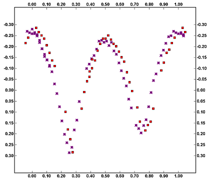
There are many methods for finding an accurate estimate of the error in the period. One is to change the period against which the data is phased by a small amount and see how well the data still fits. This can be done in MPO Canopus by changing the assumed period and regenerating the phased plot using the new period. In other programs, e.g., when using Excel to "fold the data", you would simply change the assumed period to see how much the data "spread out."

The two plots above show the data phased against the original period minus 0.02h (left) and 0.01h (right). You can plainly see that the data no longer fit very well at all – even with a shift of only 0.01h. It’s not until the shift is reduced to 0.005h that it gets difficult to see the difference between the original plot for 5.889h and the revised plot. Going by this method, a precision of 0.005h, maybe down to 0.002h would be justified.
The other method for determining precision, beyond using the error computed by the Fourier analysis routine, is based on some analytical rules. Just from general experience, Alan Harris has found that lightcurves can be “overlapped” to plus or minus a few percent of the period, depending strongly on the amplitude and on the quality of the data. To get a 1% solution, you need data overlap spaced by several cycles. To get 0.1%, you need several tens of cycles data span, and so forth. In most cases, the worry is more about the risk of missing the right number of cycles, so cycle ambiguity is the biggest concern rather than the formal uncertainty of a particular solution. The table below gives some specific examples of this concept.
|
Period
(hours) |
3
rotations (hours) 1% |
Precision (hours) 1% |
30
rotations (hours/days) 0.1% |
Precision
(hours) 0.1% |
|
2 |
6 |
0.02 |
60 / 2.50 |
0.002 |
|
5 |
15 |
0.05 |
150
/ 6.25 |
0.005 |
|
10 |
30 |
0.10 |
300
/ 12.50 |
0.010 |
|
24 |
72 |
0.24 |
720
/ 30.00 |
0.024 |
Using this table, what precision would be justified for the data for 771 Libera?
Since the two sessions were separated by four days (96 hours) and the period is about 5.9h, the asteroid rotated about 16 times between the start of the first session and the start of the second session. This is about halfway between the 3 and 30 rotations for 1% and 0.1% rotation, so a good estimate is about 0.4% precision (it’s a logarithmic scale, not linear). That translates into 0.02h. We’ve already seen that changing the period by that small amount dramatically alters the fit of the data and that it is too large an error. Since the data from both nights covers a full cycle, or nearly so, there really is no worry about finding a period other than the correct one. In this case, you can use the “sliding period” approach or use the error reported by the Fourier routine. If using the latter approach, I tend to double it, which would be 0.002h for this example, assuming that a check with the sliding period method confirms that the resulting error isn’t too small or large.