The TASS Mark IV Engineering Run

• Introduction
• Hardware
  • Cameras
  • Lens
  • Electronics
  • Mount
• Software
• Operation
• Results
• Data Mining
• Future Plans
• Acknowledgements
• References

Introduction

After two preliminary sets of hardware were built, a set of 10 triplet cameras was planned and parts were ordered. As these were the third hardware design, we called them "TASS Mark III systems". The thinking then was to set up triplet cameras spaced by one hour in RA and cover ten 3 degree wide lanes in the sky while operating the cameras in drift scan mode to look for comets.

While production of these triplets started, discussion continued on the internet. TFD soon realized that the primary problem was the software to manage all the data that these triplets would accumulate. Also, professional astronomers started to notice the plans and started to persuade TFD to think of other measurements and to include filters in the plan. The use of filters put comet discovery out of reach. To encourage their use, Bohden Paczynski kindly purchased the filters for the project. The plan was then changed. Instead of TFD operating ten triplets at his Chicago suburban location, he proposed to give them away to those interested in the project in the hope that a larger group would be able to develop the required software. The goal shifted from comet discovery to an all sky survey with emphasis on variable stars.

Seven systems were distributed under this plan and the necessary software was developed. These systems were operated over a year and a survey was completed; see "TASS Mark III Photometric Survey of the Celestial Equator" (Richmond et al. 2000) either via the ADS or at the TASS WWW site. TFD then planned a more advanced design. The Mark IV systems were designed to have about 10 times the area throughput of the Mark III systems and were more sensitive.

Seven Mark IV systems have been completed. Four have been shipped to volunteers who are operating in Cincinnati, OH, Flagstaff, AZ, Rochester, NY, and Berthoud, CO. This presentation covers only the Engineering Run of the three systems located in Batavia, IL.

Specifications

• Optics: 100 mm diameter, 400 mm focal length. Five element refractor. Coated in two bands.
• Mount: Dual Inverted Fork mount of our own design. Tangent arm RA drive.
• CCD: 2k x 2k CCD442A 15 u pixels. 80,000 e- full well. Operated in MPP mode.
• Cooling: By TEC. Cools to -40 C below chilled water temperature; usually run at -20 C with water at 20 C.
• Pixel Scale: 7.7 arc seconds
• Read Out Time: Simultaneous readout of two channels in 46 seconds.
• Declination Motion: Horizon to the pole.
• RA Motion: +/- 20 degrees from the meridian.

Hardware

From the start of the project, all were involved were encouraged to write technical notes. These now come in three classes. The Technical Notes, which now number 99, are of general interest and cover hardware details, computations on specific data sets, and everything else that does not fit in the other categories. The Show and Tell entries are what they sound like: many pictures and a few words to describe something like the construction progress to date. An example is Show and Tell 5, "Progress on the Mark IV to January, 1999." Finally there are Service Notes. These cover fixes and changes to the hardware and software. An example is Service Note 7 which covers installation of stiffener bars to improve the focus drive.

Because much of the detailed information is available in the Technical Notes files, we have just written a few words in the remainder of this section to describe the Mark IV system. You can find an overview of our design philosophy in Show-and-Tell 9.

The TASS Mark IV Camera

The cameras for the Mark IV system were designed around the CCD442A. At the time of the development (1997), these chips were being sold by Loral. The CCD design had been previously owned by Farichild, Ford and others and is now offered by Fairchild Imaging. At the time, these were the lowest-cost chips in area per dollar by a factor of two. A quite significant saving for a project with 14 cameras in service and another 18 under construction. Because of the many owners, the available data was in disarray. No two documents had the same pin labels. It was a challenge to make these chips work.

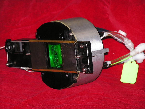
Above is the completed camera. The shutter is driven like a parlor door. It is opened in 0.2 second by a model airplane servo motor. The camera shown has a Cousins V filter. Since the camera is operated with a narrow band lens that matches the filter, the filter is never changed. The filter is thus glued permanently into the camera shell. The camera is sealed but not high vacuum tight. Dry air is circulated through the camera to prevent condensation.

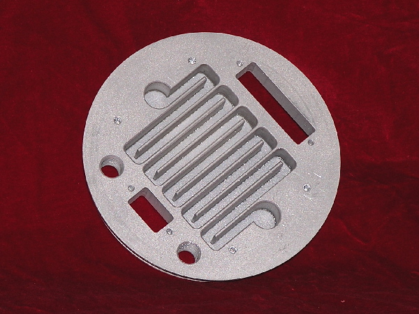
The camera is cooled by a Thermoelectric Cooler glued to a cold plate with silver filled epoxy. The plate is very thin behind the meander so that there is low temperature drop through the aluminum. A cover plate is glued over the meander and contains a pair of fittings for cooling water circulation.

The fittings are selected so that it is difficult to make the mistake of connecting the water fitting to the dry air circulation connector. This mistake was never actually made, though we made most others possible. Signal and TEC power connectors are glued into the plate. The backs of the connectors are epoxy filled to prevent leakage through the connectors. A spacer block above the TEC provides conduction to the back of the CCD. Silver filled thermal grease allows CCD removal.

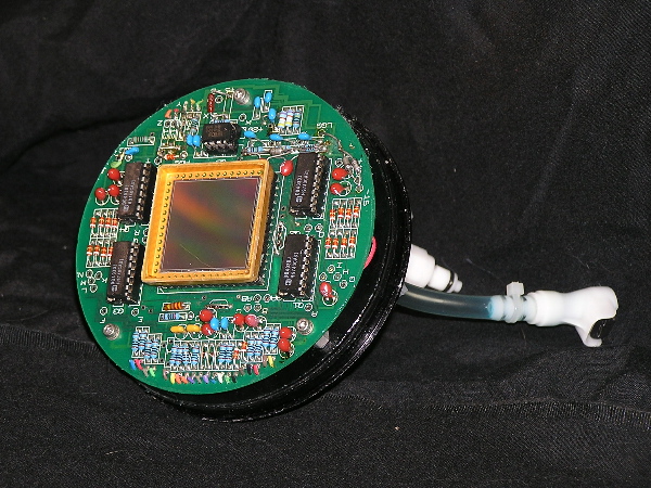
DAC generated DC voltages and logic level clocks are connected to the printed circuit board where the actual clock levels are generated by DG403 switches. A ground plane behind the socket and very short leads from the switches provides bounce free clocks which are RC shaped. The shell is sealed to the electronic assembly on the cooling plate by an "O" ring.

Additional information on the camera is available in Tech Note 40.

The TASS Mark IV Lens

We searched for some time to find a lens suitable for a wide angle survey.  One of us (TFD) kept calling specialty lens designers who quoted very expensive multi element designs.  For the most part  they were not interested in the work since they realized that the desired design was impractical.

Finally from the discussions we learned that a flat field with low coma over a wide band width was one of the design limitations.  The difficulty of the design was some high power of the bandwidth.  Realizing that one way to run a survey was to always use the same filter with a lens, we then started inquiring if narrow band lenses would be easier.  This interested Elliot Burke of High Tide Instruments who was following the list and he undertook a design at no cost. 

After a lot of computation, a design was produced that had a small number of elements (5) and which had a pixel spot size of < 1 (15u) pixel (70% energy) over the whole CCD. This compares to more expensive camera telephoto lenses that are typically down by 50% in the corners.

We do not recommend this exercise for the faint of heart.  While the lens design was done at no cost by one of the tass group, the procurement was an adventure.  There were problems with lenses that were crushed by the mount in cold weather, lenses installed backwards, and numerous errors in spacing.

We ordered 40 lenses split into 16 V, 16 Ic, 4 B, and 4 R band designs.  Elliot Burke found a clever design which used the same 5 lenses for each band but with different spacings to reduce the cost.  The lenses were coated in two bandpasses, one for the B and V lenses and another for the R and Ic. 

As noted above, there were many disasters.  Each time one occurred someone from the TASS mail list stepped forward and helped solve the problem. From a message sent to the TASS E-mail list on 3 January 1998:

"Note that this is high risk, and a lot of money for me. We want to get it right. I know this is hard. Now is the time to speak up if you know anything."

Yep!

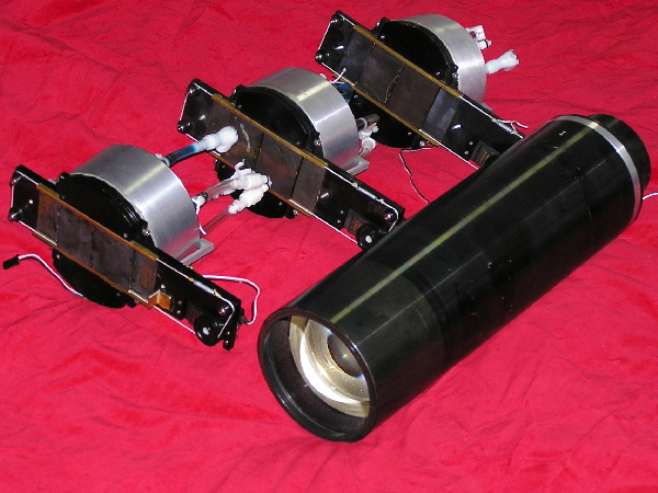
A lens shown with several cameras for comparison.  An I lens is shown.  The lenses vary in length for the various bandwidths. 

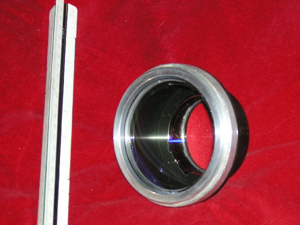
The rear cell for an I lens.  The draftsman's ruler is for comparison.  Note the non anodized ring on the lens cell.  This was required to "fix" a spacing design error.  The vendor glued the lenses in this cell and when stored in a garage over a Chicago, IL winter many of the lenses were crushed.  We had to heat the whole assembly in an oven and push out the lenses.  The cells then had to be machined to a larger radius and the lenses were mounted with RTV.

Electronics

The electronics are described in Tech Note 38

Mount

Some current pictures are shown in the Operation section below. The following technical notes give more detail:

• Tech Note 39 (early hardware)
• Tech Note 42 (the mount)
• Tech Note 69 (the RA drive)
• Show-and-Tell 1: Mark IV Construction Progress for June 1998
• Show-and-Tell 2: Mark IV Construction Progress for August 1998
• Show-and-Tell 5: Progress on Mark IV to January, 1999
• Show-and-Tell 6: Progress on Mark IV to June, 1999

Watchdog Hardware

We sleep most of the time the system is operating. Since weather is not all that predictable, we have a rain detector that closes the dome. To limit the number of bad frames that the software must eliminate, we have developed a "Clear Sky Detector" that is quite effective. This is described in Tech Note 93. When the detector does not see clear sky, dark frames are taken.

Software

The Mark IV cameras produce simultanenous pairs of images in V and I passbands. We now describe the steps by which the Mark IV reduction pipeline turns these images into lists of stars. The basic series of operations is

1. create master dark and flatfield images
2. subtract the master dark from each image
3. divide each image by the master flat
4. measure and remove the sky background
5. find stars
6. measure instrumental properties of each star
7. calibrate the position of each star
8. calibrate the magnitude of each star

Most of these steps involve pieces of the XVista suite of astronomical software, which grew out of the PC-Vista package. Our entire source code is available for anyone to use; see A pipeline for reducing TASS Mark IV data.

Creating master dark and flatfield images

We take a series of more than 10 frames with the shutter closed and lens covered to serve as "dark frames." The temperature of the camera during these dark frames is controlled to be at the same temperature as the target frames, and the exposure times are identical to those of the target frames. The pipeline creates a "master dark" frame on a pixel-by-pixel basis in the following way: the values for a given pixel are taken from each dark image, yielding a set of values which are then sorted. The mean of all values in the second and third quartiles (i.e. the mean of all values between the 25'th and 75'th percentiles) is determined, and this interquartile mean is placed into the output "master dark" at that pixel location.

To create a "master flatfield" frame, we can use either the target images themselves or a set of special images of a diffuse light source; we typically use approximately 30 target frames from a good night. Before the frames are combined, the dark current is removed from each one. Because the temperature of the camera may have changed slightly during the hours separating the dark frames from the target frames, we examine a set of prescan columns at the edge of the frames to look for an offset between the master dark image and each raw flatfield image; we add a constant to all pixels in the raw flatfield frame to remove any offset. We then subtract the master dark from each raw flatfield frame to remove the dark current. The dark-subtracted flatfield frames are then subjected to the same pixel-by-pixel interquartile mean to generate a "master flatfield" frame. We trim the edges from this master flatfield so that only pixels struck fully by light remain.

During the early stages of our work, we found a number of bad spots in the images from each camera. Some are always present, caused by defects in the CCD chip; others occur rarely, when moisture leaks into the air near the chip and freezes into ice crystals on the silicon. These bad spots are easily seen on the master flatfield images, so we devised a scheme to identify them. We search for regions of connected pixels in the master flatfield frame which all lie far from the local mean value. We store a list of all such bad regions as the "mask" corresponding to each camera. We will later set a flag in all measurements made in any "masked" region.

Experience has shown us that the flatfield frames are nearly identical from one night to the next, so we use a single "master" flatfield frame for each camera over a period of a month or two.

Subtracting the master dark frame from each target image

The first step in the reduction of each raw target frame is to remove the dark current. We compare a set of prescan columns at the edge of each image to the same prescan columns in the master dark frame, and shift all pixels in the target frame by a constant value to remove any difference. We then subtract the value of the master dark frame from the target frame on a pixel-by-pixel basis.

We note a small, systematic error which occurs at this point due to the limitations of our software. The XVista package works on 16-bit integer FITS files only. Although the raw images have a dynamic range which spans 16 bits, this subtraction truncates the data so that it lies within 15 bits (pixel values ranging from 0 to +32,767). In theory, this could cause very bright stars to appear artificially faint, since pixel values of, say, 50,000 counts above the dark current would be set to 32,767 counts. We believe that this issue is not particularly significant in practice for two reasons: first, the full-well capacity of the CCDs is 80,000 electrons, and we run the devices at a gain of 2.5 electrons per data number. Thus, any pixel value above 32,767 is very near full-well and probably non-linear anyway. Second, we mark any such pixel values as suspect, and mark their magnitudes in our output as well, so we can remove them from later analysis.

Dividing each image by the master flat

We divide the dark-subtracted images pixel-by-pixel, by a normalized version of the corresponding master flatfield image. The resulting clean images are trimmed to remove prescan and overscan columns, and the very top and bottom rows which are not fully illuminated.

Measuring and removing the sky background

We measure the "sky" value for each image by forming a histogram of all pixel values, finding the peak of the histogram, and fitting a gaussian to the region near the peak. This procedure gives us a notion of both the mean background value and its standard deviation. We have found that both measures can be used to distinguish good nights from cloudy ones. The user can set limits on both quantities for each camera, so that any image failing to fall within the limits is automatically marked as "bad."

There are times when our "clean" images show clear spatial variations, sometimes due to passing clouds, sometimes due to transient lights from neighboring houses. Since our method of finding stars assumes a uniform background value across the entire frame, we try to remove large-scale variations at this point. We divide the frame into a rectangular grid of sub-frames and estimate the background value of each sub-frame by fitting a gaussian to the histogram of its pixel values. We then fit a first-order polynomial to this grid in each direction, defining a model for the background which varies smoothly across the entire image. We subtract this model from the image, then re-calculate the mean and standard deviation of the "sky" as described above.

Finding stars

We search for stars in each cleaned image by defining a large set of candidates and then passing them through a set of tests. The first step involves a simple threshold based on the sky values: any pixel which exceeds the mean sky value by more than a given number (typically 3 ) of standard deviations marks a candidate. The properties of nearby pixels -- full-width at half-maximum (FWHM), roundness and sharpness (see Stetson 1987) -- are calculated and subject to a series of tests. Any candidate which passes all the tests is designated a star.

We keep track of the number of stars found in each image. If the number is either too big or too small, we mark the image as "bad." A good image typically contains several thousand objects which pass all our tests.

Measuring instrumental properties of each star

We calculate the (row, col) position of each star by fitting 1-D gaussians to the intensity-weighted marginal sums of pixel values in each direction.

We calculate the instrumental magnitude of each star using aperture photometry, with the same circular aperture for all stars on a frame. We add up the light from all pixels within a circular aperture of radius typically 30 arcseconds (i.e. 4 pixels); for pixels which lie partially within the circle, we take a fraction of the intensity equal to the fraction of the area within the aperture. We then find a local sky value for each star by determining the median of all pixels values within an annulus around the star with typical radii 77 to 154 arcseconds (i.e. 10 to 20 pixels). We subtract the local sky's contribution to the light within each aperture, and convert the result to an instrumental magnitude. We also estimate the uncertainty of this magnitude based upon the photon statistics of both the sky's light and star's light.

The list of instrumental positions and magnitudes for objects found within each frame also contains a set of flags. We set one flag for any star which contains sky-subtracted pixel values above a particular threshold, which mark it as "possibly saturated." We set different flags for stars which fall near the edges of the frame, or close to one of the regions marked as "bad" in the image mask.

Calibrating the positions of stars

In order to convert our (row, col) positions of each star into (RA, Dec), we use a set of stars from the Tycho-2 catalog (reference) as a reference. There are typically 40-60 bright Tycho stars per image. Our match software

1. projects all measured (row, col) positions around the center of each image onto a tangent plane,
2. projects the (RA, Dec) positions of all Tycho stars around the estimated position of each image onto a second tangent plane
3. searches for matches between the two sets of points
4. defines a cubic transformation between the two sets of points
5. applies the transformation to the projected positions of all stars
6. de-projects the transformed positions into (RA, Dec)

If the routine cannot find a match between the two sets of points (due to clouds or a pointing error), it discards the frame from all further processing.

When we compare the resulting positions to those in the Tycho-2 catalog, we find a standard deviation of roughly 0.6 arcsecond for bright stars (V < 10) and roughly 1.2 arcseconds for faint stars (V > 10).

Calibrating the magnitudes of stars

In order to convert our instrumental magnitudes to some standard scale, we again use Tycho-2 as a reference catalog. However, we first create a "photometric subset" by selecting only stars with the following properties:

• 1 < Bt < 11.8
• 1 < Vt < 10.7
• -0.2 < (Bt - Vt) < 1.8
• sigma(Bt) < 0.05
• sigma(Vt) < 0.05
• no other Tycho-2 star within 50 arcsec
• no indication of binarity in Tycho-2 entry

We then apply a set of linear transformations to the Tycho-2 photometry (Henden, reference private communication) to convert Bt and Vt to Johnson-Cousins V and I. We then compare these approximated V and I magnitudes to the instrumental measurements of stars in our images.

We begin by collecting matching instrumental measurements of stars from the simultaneous V and I images; stars which are detected only in a single passband are discarded. We create a photometric solution for each night in the V passband like so:

     calibrated   V  =      v     +  a   +   b * (v - i)  -  k * airmass
                                      j
  

where v and i represent raw measurements, V the calibrated magnitude, a_j the zero point for frame j during the night, and k an estimate of the first-order extinction coefficient. In other words, we allow the zero-point to change from one image to the next (due to clouds), but force a single color term b for the entire night. The extinction coefficient k acts only differentially within each frame; since our images span almost six degrees diagonally, the differential extinction can become significant, especially in V-band. We are unable to solve for extinction, but even a rough guess will reduce the differential effect substantially.

We create a similar photometric equation to transform the instrumental I-band measurements to the Tycho system. We solve each equation via linear least-squares techniques. The resulting output values for the zero-point coeffients and color term give us another indication of the quality of a night, which we can use to disqualify all or part of its measurements from further consideration.

The output of the pipeline is a set of star lists, one per simultaneous pair of images, containing the (RA, Dec) position and (V, I) magnitudes of each star in the image. A good night yields several thousand stars per image and several hundred images; the best nights have produced almost two million pairs of magnitudes.

Operation

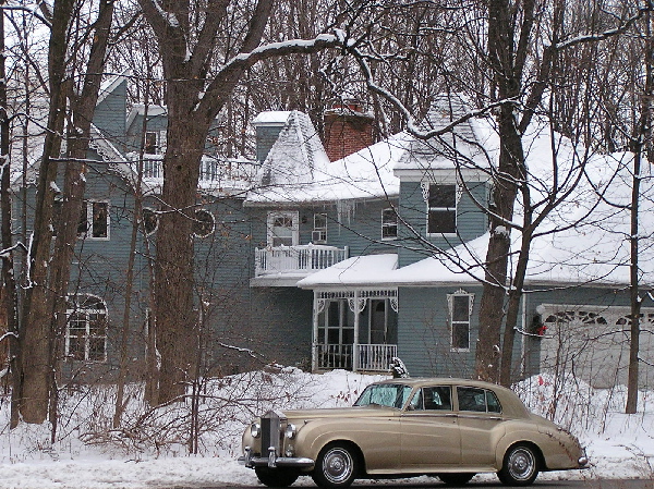
The dome containing TOM2 and TOM3 is on the shed roof in the upper left corner of this picture. TOM1 is in the tower at the center to the left of the chimney. A third floor level deck connected by a spiral staircase allows access to the various cameras.

We are able to take data about 100 nights a year here in suburban Chicago. During the day we scan the weather reports to see if the night will be possibly clear enough to take some data. Near dusk we open up the dome and the tower. The chilled water pumps and dry air pumps are started and the cameras set to cool down mode. It takes about an hour for the temperature to stabilize. Since we control the temperature of the cameras to less than 1 C, we find that the difference in darks from night to night is much less than the sky noise. After trying various light boxes, screen flats, fog flats, and the like, median sky flats are used. These are made from clear sky data runs. This means that darks and flats are not a part of the normal run procedure. We plan to do them several times a month for the coming run.

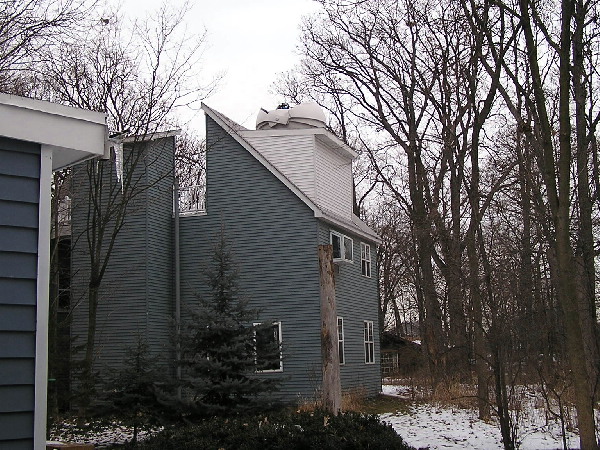
A better view of the 7-foot diameter clam shell dome that houses two dual systems.

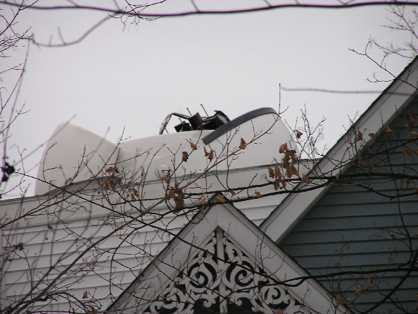
A closeup of the dome. One can see one of the telescope pairs pointing to the upper left. (South)

Shortly before it is fully dark, the night's image run is started. The three systems are set to scan images in Declination. TOM1 scans from -4 to +16 degrees in 6 steps of 4 degrees. TOM2 scans +20 to +48 in 8 steps of 4 degrees and TOM3 scans from +52 to +88 in 10 steps of 4 degrees. With 90 second exposures and 46 seconds read out and adding motion time we get about 20 V and Ic exposures from each camera pair each hour of operation. This is a raw data rate of 1 GByte an hour. The rate is just sufficient to cover all the sky that transits the meridian during the operating night. Once it gets dark enough to get images we examine a few over the ethernet connection from our office. Then with an eye to the weather, we go to bed. At dawn, the dome is closed and TOM1 is pushed into it's enclosure. The data analysis pipeline is then started which copies all the data from the three camera control computers into the 6 processing computers. This is done over a standard eathernet connection which links the 3 data collection computers running Windows to the 6 data processing computers running Linux.

The operator then goes back to bed. Sometimes a few images are examined if somehow the operator really wakes up.

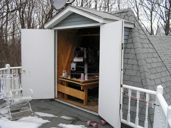
TOM1 in its tower with the doors open.

At an hour reserved for retired folk, the operator gets out of bed and does some checks on the data quality. Five to 10% of the images are examined and some assessment is made as to whether the data is worth keeping. This examination continues at intervals through the day. It takes 12 to 14 hours for the slowest (1.5 GHz Pentium) to complete the processing so it is near time to start running again by the time processing is complete. Since the data is copied to the processing computers, the processing step can take up to 24 hours before it would fall behind. Computers being what they are, the pipeline sometimes does not run or a computer has died or ... After the processing is complete, the images that passed the cuts are written to CD. This is usually done late in the evening, sometimes after the next run has started. The result of the processing is written to a monthly file and a backup file on a different computer. The processing result is a list of stars with their magnitudes and positions as well as control data which records the conditions of the run, software version, etc...

At the end of each month, the accumulated measurements are written to four sets of CDs. One set is mailed to the on line data base at http://sallman.tass-survey.org/servlet/markiv/

A second set is mailed to the web site at http://www.tass-survey.org/tass/tass.shtml as backup, and a master set and a backup set are kept at the data collection site in Batavia, IL.

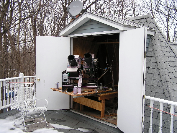
TOM1 with the coo-coo clock mount pulled out ready for operation.

Results

We have collected over 77 Million V, Ic measurement pairs of 8.2 Million stars in the northern hemisphere to -6 degrees.  We have measured 2.6 Million stars at least ten times.  Many stars have been measured several hundred times.   

Coverage for at least one measurement in V and Ic.  Declination from -6 to +90, RA 0 to 360 degrees. 

Above is the coverage for at least one measurement pair.  We only keep data for which there is a simultaneous detection in the V and the Ic filters.  This causes complete loss of the data point when one of the filters drops below the detection limit of around magnitude 15..  When, as in very red stars, there is a large difference this sometimes causes loss of data when a star is quite bright in the other filter.

Coverage for at least ten measurements in V and Ic.  Declination from -6 to +90, RA 0 to 360 degrees. 

Next is the coverage for at least ten measurements.  Some structure can be noted which is due to the overlap of the measurement frames.  There are problems due to the overlap of the fields. 

Plot of stars in a small portion of the survey area which a) were measured more than 40 times in V, and b) have standard deviation from the mean greater than 0.1 mag. Overlap effects can be seen in Declination, and to a lesser extent in RA, due to the non-random pattern of pointings.

The overlap problems are further illustrated in the plot above where we show stars that are measured more than 40 times in V and where the sigma of the measurements of the individual stars is > 0.1.  It is obvious that the error is greater in the field overlap area.  For some of the camera pairs, we have detected and corrected a N-S tilt that could cause this.  Of greater suspicion is the quality of the sky in suburban Chicago. 

Small area data plot for stars measured 40 times or more where the sigma of each star's measurements is < 0.1.

Next we show a subset of the 40 sample or more V data where we selected stars where the sigma of the measurements of the star was < 0.1.  The scatter is clearly lower in the areas where the frames do not overlap.  More detailed studies of the errors in the data can be found in the technical notes.  For example, Tech Note 97 and Tech Note 98.

To show an overall view of the scatter of the data, we plot the sigma for stars measured 3 times or more averaged in 0.1 magnitude bins.   This is shown first as a log plot. 

A log plot showing scatter in the measurements of stars measured 3 or more times in V in 0.1 magnitude bins. 

On a log plot we expect a linear rise in scatter due to the statistics of the measurement.  This can be seen to start roughly at magnitude 11.  Below magnitude 11, something else limits the scatter to around magnitude 0.05.  We know this is due to variation of the position in the frame since in selective tracking experiments the noise floor is below 0.01 sigma.  For example, figure 5 and 6 of Tech Note 88.

Since we have not excluded variables stars from this data, a small part of the scatter is due to measurement changes that are real. 

This same data is next plotted in a more conventional linear plot.

A linear plot showing scatter in the measurements of stars measured 3 or more times in V in 0.1 magnitude bins.

We continue to study the data.  We have been converting all the systems to be identical and will shortly start taking additional data to compare to the data presented here.  We have some hope to isolate the limitations on the scatter. 

We observe however, that this data will be mostly useful from about magnitude 11 to 13.  The brighter stars are well measured.  In the useful range the scatter appears to be limited by statistics. 

Data Mining

There is a lot of day to day work running this survey. For amusement in off hours, we have hunted the data for variable stars. There is a lot of work yet to be done on programs to do this. The result of an early effort contains 1713 variable star candidates in a format that can be submitted to VizieR. Depending on our skill in writing the search program often less that half turn out to be known variable stars. The rest are mostly obvious variables. Our emphasis has been to develop the catalog of information. We put our "finds" on the mail list or on the Wiki and encourage others to study these stars. Several have taken our preliminary data, observed the star, taken enough data to confirm the variability type, and published the data (e.g., Koppleman and Terrell 2002; Koppelman and West 2002; Wils and Greaves 2003; Wils 2003). This is very encouraging for us. By acting as only a source of information and not claiming all the credit, we have encouraged a number of enthusiasts to follow the tass work and to add greatly to the overall effort.

To give some idea as to the nature of this data, we have selected 10 stars from the candidate list and show them below. For selection, we simply paged through the list stopping at random and marked a star. The selected stars were run through VizieR using just the General Catalog of Variable Stars. These stars may be on other lists.

First, for comparison, we show a couple of stars picked for having more than 50 measurements and which were not on the variable list. The magnitude scale is set to be similar to the later events for comparison.

Below: RA 05:30:51.5 Dec -00:08:09

Below: RA 07:32:32.7 Dec -01:00:58

Next we show the ten stars selected from the potential variable list. The data points are connected to aid one of us (TFD) who has a minor visual impairment. The vertical axis is magnitude with the Ic filter plotted in red and the V filter plotted in green. The horizontal axis is Julian Day minus 2,450,000. The label is the star's position as TASShhmmss+ddmmss.

Below: RA 00:30:08.5 Dec +37:53:34. A probable long period variable.

Below: RA 01:09:44.5 Dec -02:02:31. A probable short period variable.

Below: RA 01:37:41.5 Dec +07:03:19. A probable short period variable.

Below: RA 06:12:26.9 Dec +12:12:36. This is EI Ori, a carbon star.

Below: RA 07:03:54.0 Dec +11:01:42. A probable short period variable.

Below: RA 07:17:10.2 Dec -01:44:17. This is V0634 Mon, an eclipsing variable with period 2.11 days.

Below: RA 08:06:21.6 Dec +03:23:02. No obvious classification. More data is needed!

Below: RA 13:51:50.8 Dec -02:12:30. A probable short-period variable.

Below: RA 15:00:53.4 Dec -01:23:54. A probable long-period variable.

Below: RA 20:13:46.1 Dec +02:59:31. This is V0517 Aql, a Mira variable.

Future Plans

A design is in process for a Mark V. This has been designed as a 4 camera mount with the capability of tracking longer than the Mark IV s. We would use this design to take long runs tracking the sky in four filters to obtain data on short period variables.

Acknowledgements

References

• Greaves, J., and Wils, P., 2003, Confirmation of Variability of FASTT Suspected Variables IBVS 5458, 1
• Koppelman, M. and West, D., 2002, NSV 10892 is a W UMa Eclipsing Binary , IBVS 5327, 1
• Koppelman, M. and Terrell, D., 2002, GSC 00279-00321: A New W UMa Eclipsing Binary IBVS 5299, 1
• Richmond, M. W. et al., 2000 TASS Mark III Photometric Survey of the Celestial Equator PASP, 112, 397
• Stetson, P. B., 1987, DAOPHOT - A computer program for crowded-field stellar photometry PASP 99, 191
• Treffers, R. R. and Richmond, M. W., 1989 PCVISTA: A Library of Astronomical Image-Processing Programs for the IBM PC, PASP, 101, 725
• Wils, P., 2003, Confirmation of Variability of Bidelman-MacConnell Suspected Variables IBVS 5457, 1

Readers can find most of the web-based information discussed above by starting at

• The main TASS home page
• The TASS Mark IV Engineering Database, created and run by Michael Sallman
• The TASS Wiki, run by Peter Mount, with large contributions from Patrick Wils

Last modified by MWR 3/25/2004

Enter the forum and ask your questions to the author!

Back to the Meeting index